Here are my go-to Excel techniques that, time and again, make my work easier, more efficient, and sometimes even fun! These tips are not exclusively for nonprofits, by any means; they are used in business all the time too.
I’ve included links to help resources for each tip, using a variety of different Excel help sites. Mostly I point you to sites describing how to do these things in Excel 2010, but you can expect some of the examples to look a bit different than how your version of Excel may look.
If you are new to Excel and prefer a more basic introduction, I’d recommend DeskBright, where you can learn basic Excel skills and ask questions in a user forum.
Keyboard Shortcuts. Heavy Excel users get kind of obsessed with saving keystrokes and avoiding the mouse. I’m sure I use only a fraction of what’s available, but the keyboard shortcuts are something I can’t live without (as I realized when I was trying out Numbers for Mac and these time-saving keystrokes weren’t readily available). Here are some easy ones to start with:
– End followed by Arrow Key: places your cursor at the last cell of an uninterrupted row or column (i,e., stops at blanks)
– Shift, and then End followed by Arrow Key: same as above, but you’ll select all the cells
– Command + Home (Mac) or Ctrl + Home (PC): places your cursor at the very top left position in your sheet
– Ctrl + PgDn (Mac or PC): moves you to the next sheet in your workbook (PgUp moves you to the left)
Many more shortcuts: http://office.microsoft.com/en-us/excel-help/keyboard-shortcuts-in-excel-2010-HP010342494.aspx
Filter. When you apply a filter to your spreadsheet, which you do by selecting a header row and then clicking the Filter button, you can open a dropdown box on the header of any column and select which values in that column you want to filter on. Excel handles large sets of dates very nicely, automatically rolling up by month and year. This is a terrific way to cut down the amount of data you need to be looking at. There is, however, one critical mistake to avoid: Don’t block and copy when you’re in Filter mode; you will most likely fill in cells that you can’t see, which that are located between the exposed rows of data.
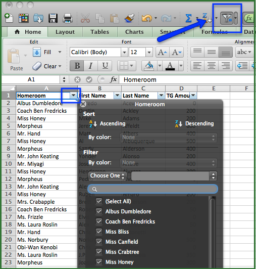
More help: http://www.wikihow.com/Use-AutoFilter-in-MS-Excel
Vlookup. This is probably the single most useful tip I can share. When my team at Amazon.com discovered this Excel feature back in 1999 it made us giddy with excitement. You use vlookup when you have two spreadsheets and you want to merge data from one of them into the other one. For example, maybe you have one spreadsheet with name and contact information, but you have gift history in another spreadsheet. You need a column that is shared between the two. A unique identifier column is ideal, but you could also use email address, name, or any other unique ID. In brief, for each row of the receiving spreadsheet, you can look up the value from one of the columns in each row and report back a different column from the other spreadsheet.
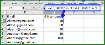
In the example above, we’re in Sheet 1 and we’re referencing a different spreadsheet (Sheet 3) where we are looking up an email address (P2). In Sheet 3, we find the email address (i.e., AllenSt@gmail.com) and pull back an associated value from the other spreadsheet (the value we’re pulling back is “50”). The “2” in the formula means to pull back column 2, starting from the reference column, and the “false” is just something you have to put in there without asking why 🙂
More help: http://www.techonthenet.com/excel/formulas/vlookup.php
And: http://spreadsheeto.com/vlookup/ (published in 2016)
Trim: The trim feature cuts out excess spaces around the text in a cell. This could be a crucial help if you’re trying to run a vlookup on a cell but aren’t finding a match when you expect to find one. That could be because in one case the text is “John” and in another case it’s “John ” (with a space). Use trim to cut out the excess spaces and your vlookups will run much more smoothly.
- Concatenate. This is a simple way to combine the values of two or more cells into another cell. For example, if you have columns for First Name and Last Name and want to create a Full Name column, you can combine the values from the first two columns into a third. If First Name and Last Name are in columns A and B, then in column C, starting on row 2, your formula would be “=concatenate(a2,” “,b2)” or for a shorthand version, it can be simply “=a2&” “&b2”. Note that you have to add a blank space, otherwise the names will run together.
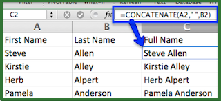
In the example above, we are combining the contents on row 2 from columns A and B into cell C2.
More help: http://office.microsoft.com/en-us/excel-help/concatenate-function-HP010062562.aspx. - Text to Columns. If you have text that you need to split up into component parts, then text to columns is a great solution. Taking the above example in reverse, you might have Full Name in a column and you want to split that into separate columns for First and Last Name. You can tell Excel to split on spaces or any number of other identifiers. If you have a mix of two and three piece names, you’ll run into some difficulty, because Excel will split a three-piece name into three columns. I usually then sort by that third name column, so I can edit those rows the way I need to.
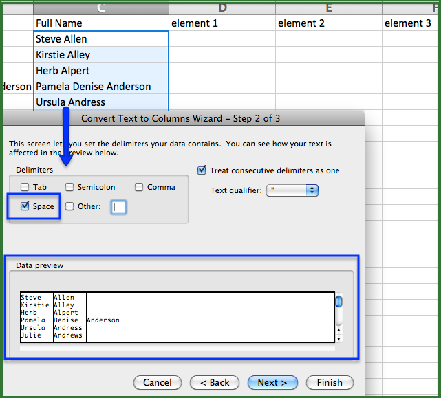
Above we’re telling Excel to split the value of the data in column C wherever a “space” appears. You want to make sure you have blank columns available to the right, because that’s where Excel will place the split out values.
More help: http://www.excel-easy.com/examples/text-to-columns.html - Conditional Formatting (for duplicates). In Excel you can format the cells of a column based on rules you select. This can help you quickly identify highs and lows in a column, but I mostly use it to help me find duplicate values. Then, I like to sort on the cell color to get all my duplicates grouped together, and further sort by the values in the column to get the exact matches right next to each other.
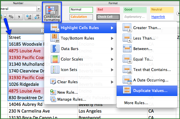
Above we’ve highlighted a set of cells and then clicked the Conditional Formatting icon and told Excel to format the cells that contain a value that is duplicated somewhere in the selected set of cells. This could, for example, help you find two people that share the same address.
More help: http://www.tech-recipes.com/rx/35290/excel-2013-find-duplicate-data-using-conditional-formatting/ - Remove Duplicates. There are many times that I need to get just the unique values from a list. For example, I might have a long list of possible constituent attributes in my spreadsheet and I need to get the list of the attributes used. For this, I copy the column to a new part of my spreadsheet and run the Remove Duplicates feature, which reduces my column to just unique values.
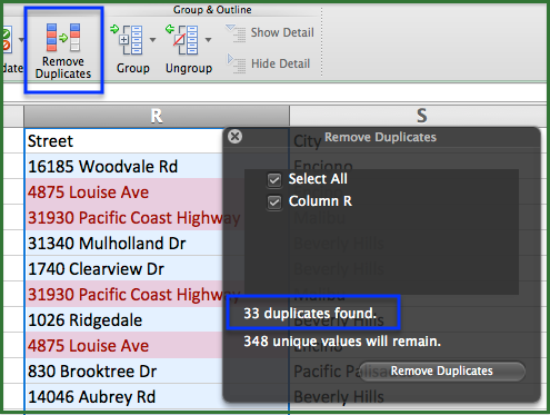
If we click the Remove Duplicates button above, the values in column R will be reduced by 33.
More help: http://www.rosebudtech.com/windows-8/removing-duplicate-data-from-your-spreadsheet-excel-2010/ - If, then. The “If, Then” statement in Excel can make you feel like a computer programmer, even if you have no Visual Basic skills. You can nest multiple “if, then” statements inside one another to create some pretty complex logic. In brief, the formula includes a criteria and then tells what to do if that criteria is met and then what to do if the criteria is not met. Let’s imagine you have a column of donation totals and you want to assign people to a Giving Tier based on those totals. Your top tier might be for people who’ve given over $50,000 and we’ll call that our Gold level. The “if, then” statement would be simply:=if(B2>50000,”gold”,””). This tells Excel to put the word “gold” into the cell where you place this formula if the cell B2 has a value of greater than 50000. If B2 does not meet that criteria, we’re telling Excel to leave the cell blank (which is best accomplished by the double quotation marks). In the example below, we have additional tiers.
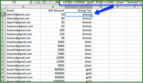
To keep things simple, we’ll have a tier for $1,000 through $50,000 and then one for below $1,000. Here’s what the full “if, then” statement would look like: =if(B2>50000,”gold”,if(B2>1000,”silver”,”bronze”). You would read this statement as, “if cell B2 has a value of greater than 50,000 then enter the word “gold” otherwise, if it has a value over 1,000 put in the word “silver” and if neither of those is true, put in the word “bronze”.
More help: http://office.microsoft.com/en-us/excel-help/if-function-HP010342586.aspx - Macros. This is a bit beyond my comfort zone and reminds me why I never became a computer programmer 🙂 But if you can get Macros to work, they sure save a lot of time. Basically they do repetitive tasks, so instead of doing lots of the same key strokes over and over again, you can run a Macro (with a single keystroke). My colleague Nick sent around a macro he uses to remove columns from spreadsheets that have nothing in them (except the header). I was able to successfully implement this on my PC but not on my Mac. I also had to save my Excel file as a Macro-enabled workbook (*.xlsm) before it would work. Here’s the code, which you want to drop into a Macro script editor, between the start and end lines:
—————————————————————————————————
first = Selection.Column
last = Selection.Columns(Selection.Columns.Count).Column
For i = last To first Step -1
If WorksheetFunction.CountBlank(ActiveSheet.Columns(i)) = 1048575 Then
Columns(i).Delete
End If
Next i
—————————————————————————————————
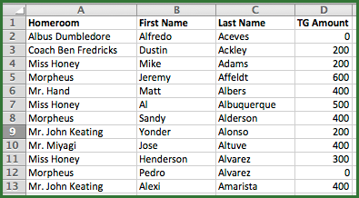
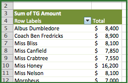
More help: http://chandoo.org/wp/2011/08/29/introduction-to-vba-macros/ - Pivot tables. This is a great way to run summary reports. In brief, pivot tables let you define which sets of data should be used to create the horizontal and vertical values by which you want to sum your data. OK, now in plain English: let’s say you have a spreadsheet with homeroom teacher names in column A, students in B and C, and giving amounts in column D. You want to know the total for each homeroom. A pivot table can do that quickly and easily.
Raw data:
Pivot table:
More help: http://www.dummies.com/how-to/content/how-to-create-a-pivot-table-in-excel-2010.seriesId-223716.html

